Seeing a Row and Its Neighbours: Window Functions
The OVER clause that computes across a set of rows without collapsing them — how a window differs from GROUP BY, and how ROW_NUMBER, RANK, DENSE_RANK, and NTILE each handle a tie. Run against PostgreSQL 18.
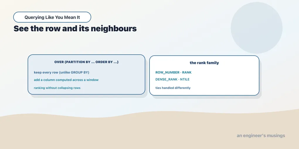
Aggregation, back in Series 1, has one property that is sometimes exactly wrong: it destroys rows. GROUP BY genre turns a hundred books into one summary line, and the hundred books are gone. But a huge class of real questions needs the summary and the rows at the same time. “Show me each book with its rank in its genre.” “Show me each order next to the customer’s running total.” You can’t answer those with GROUP BY, because the answer has one row per book, not one per genre.
Window functions are the fix, and they’re the single most useful thing in this series. A window function computes a value across a set of related rows — a window — and attaches it to each row without collapsing anything. Same number of rows out as in, plus a new column that saw the neighbours. This chapter introduces the idea and the ranking functions; the next two chapters push it much further.
The OVER clause
A window function is an ordinary function followed by OVER (...). The OVER clause defines the window — which rows this row gets to see. It has two optional parts:
PARTITION BYsplits the rows into groups, likeGROUP BY, but the groups aren’t collapsed. The function restarts for each partition.ORDER BYorders the rows within each partition, which matters for anything rank- or position-based.
Rank the books in a genre by price, highest first:
WITH ranked AS (
  SELECT genre, title, price,
         ROW_NUMBER() OVER (PARTITION BY genre ORDER BY price DESC) AS rn
  FROM books
  WHERE genre IN ('Poetry', 'History')
)
SELECT genre, title, price, rn
FROM ranked
WHERE rn <= 3
ORDER BY genre, rn;
genre | title | price | rn
---------+----------------+-------+----
History | Book Title 69 | 53.37 | 1
History | Book Title 171 | 53.06 | 2
History | Book Title 315 | 52.72 | 3
Poetry | Book Title 527 | 54.59 | 1
Poetry | Book Title 83 | 54.38 | 2
Poetry | Book Title 131 | 53.57 | 3
(6 rows)ROW_NUMBER() OVER (PARTITION BY genre ORDER BY price DESC) reads as: for each genre, number the books 1, 2, 3… from most expensive down. The numbering restarts at each genre: History has its own 1, Poetry has its own 1. That’s because PARTITION BY genre gave each genre its own window. Every book keeps its row; the window just added a column. (I wrapped it in a CTE and filtered rn <= 3 because a window function can’t be used in the same query’s WHERE — it’s computed too late in the pipeline. That “filter the ranked rows in an outer query” move is the top-N-per-group pattern. Chapter 5 gives it its own treatment.)
Why this isn’t GROUP BY
The contrast is the whole point, so make it concrete. Ask the same underlying question with GROUP BY:
SELECT genre, max(price) AS top_price, count(*) AS books
FROM books
WHERE genre IN ('Poetry', 'History')
GROUP BY genre
ORDER BY genre;
genre | top_price | books
---------+-----------+-------
History | 53.37 | 100
Poetry | 54.59 | 100
(2 rows)Two rows. GROUP BY folded a hundred books per genre into a single summary. You get the top price, but you’ve lost every individual book: you can’t say which title it was, or what the second and third places were. The window version kept all hundred rows per genre and stamped each with its rank. That’s the trade: GROUP BY when you want the summary instead of the rows, a window function when you want the summary alongside the rows. Reach for a window whenever a question sounds like “each row, plus something about its group.”
Four ranking functions, and the tie
ROW_NUMBER is one of four ranking functions, and the difference between them only shows up on ties — rows the ORDER BY can’t tell apart. Book prices are nearly all distinct, so ties are hard to see there. Order counts per customer are integers, and plenty of customers tie. Here are the top twelve customers by lifetime order count, with three ranking functions side by side:
WITH cust_orders AS (
  SELECT customer_id, count(*) AS n_orders
  FROM orders GROUP BY customer_id
)
SELECT customer_id, n_orders,
       ROW_NUMBER() OVER w AS row_number,
       RANK()       OVER w AS rank,
       DENSE_RANK() OVER w AS dense_rank
FROM cust_orders
WINDOW w AS (ORDER BY n_orders DESC)
ORDER BY n_orders DESC
LIMIT 12;
customer_id | n_orders | row_number | rank | dense_rank
-------------+----------+------------+------+------------
3549 | 29 | 1 | 1 | 1
2976 | 25 | 2 | 2 | 2
4850 | 24 | 3 | 3 | 3
1840 | 24 | 4 | 3 | 3
409 | 24 | 5 | 3 | 3
1820 | 24 | 6 | 3 | 3
3247 | 24 | 7 | 3 | 3
300 | 24 | 8 | 3 | 3
2969 | 24 | 9 | 3 | 3
4339 | 24 | 10 | 3 | 3
4226 | 23 | 11 | 11 | 4
1507 | 23 | 12 | 11 | 4
(12 rows)Eight customers tie at 24 orders, and that’s where the three functions split:
ROW_NUMBERnever ties. It assigns 3, 4, 5, 6, 7, 8, 9, 10 to the eight tied customers: distinct numbers, in an order Postgres picks arbitrarily among the ties. Use it when you need a unique sequence and don’t care how ties break — deduplication, pagination, “give me exactly one per group.”RANKgives every tied row the same rank — all eight are3— and then skips. The next customer down is rank11, not4, because ranks 4 through 10 were “used up” by the tie. This is standings-style ranking: a leaderboard where eight people tie for third and the next is eleventh.DENSE_RANKalso gives the ties the same rank (3) but does not skip: the next distinct value is rank4. No gaps. Use it when you want “how many distinct values are above this one,” not “what position is this.”
That’s the entire distinction, and it’s worth committing: ROW_NUMBER breaks ties, RANK keeps ties and leaves gaps, DENSE_RANK keeps ties and closes gaps. (I also used a named WINDOW w AS (...) clause so all three functions share one window definition, instead of repeating OVER (ORDER BY n_orders DESC) three times. Pure convenience, and handy once several columns share a window.)
NTILE: cutting into buckets
The fourth ranking function, NTILE(n), splits the ordered rows into n roughly equal buckets and labels each row with its bucket number. It’s how you compute quartiles, deciles, or “top third.” Here are the nine months of 2025 by order volume, cut into three tiers:
WITH monthly AS (
  SELECT date_trunc('month', order_date)::date AS month, count(*) AS orders
  FROM orders WHERE order_date >= '2025-01-01'
  GROUP BY 1
)
SELECT month, orders,
       NTILE(3) OVER (ORDER BY orders DESC) AS tier
FROM monthly
ORDER BY orders DESC;
month | orders | tier
------------+--------+------
2025-08-01 | 1927 | 1
2025-01-01 | 1882 | 1
2025-04-01 | 1865 | 1
2025-05-01 | 1862 | 2
2025-03-01 | 1855 | 2
2025-07-01 | 1838 | 2
2025-06-01 | 1784 | 3
2025-02-01 | 1670 | 3
2025-09-01 | 1641 | 3Nine months, three tiers of three: the busiest three land in tier 1, the middle three in tier 2, the quietest three in tier 3. When the row count doesn’t divide evenly, NTILE makes the earlier buckets one row larger. Unlike RANK, NTILE ignores ties entirely — it fills buckets by position, so two rows with the same value can fall on either side of a boundary. It’s about equal-sized groups, not equal values.
All four ranking functions are standard SQL. They work in Postgres and in every other database that has window functions: SQL Server, Oracle, modern MySQL 8, and SQLite all support them. That portability is real, unlike a lot of SQL.
Final thoughts
A window function computes across a set of related rows and attaches the result to each row without collapsing it — the thing GROUP BY structurally cannot do. OVER (PARTITION BY … ORDER BY …) names the window: PARTITION BY restarts the function per group, ORDER BY sequences the rows inside it. The four ranking functions differ only on ties, and the difference is worth knowing cold. ROW_NUMBER forces uniqueness. RANK leaves gaps after a tie, DENSE_RANK doesn’t, and NTILE slices into buckets by position. So far we’ve only ranked, which uses the order of the window but not really its extent. Next we control exactly which rows the window spans — the frame — and that unlocks running totals and moving averages.
Comments