Three Ways to Meet in the Middle: How Joins Actually Run

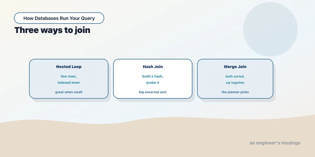
You’ve written hundreds of joins by now, and every one of them looked the same: JOIN ... ON. The word JOIN is a request, not an instruction. It says match these rows by this key, and leaves the how to the database, exactly like the rest of SQL. But underneath, there are only three real ways to match two sets of rows. The difference between them is the difference between a query that returns in 4 milliseconds and the same query taking 400. This chapter is about those three algorithms, when each one wins, and how to watch the planner choose.

Everything here was run against PostgreSQL 18 on the bookshop, and the plans are pasted in as they came back.

The three algorithms

Nested loop. For each row on the outer side, look up the matching rows on the inner side. If the inner side has an index on the join key, each lookup is cheap, and the whole join costs about (outer rows) × (one index lookup). This is the join you want when the outer side is small, or highly filtered, and the inner side is indexed. It is terrible when both sides are large, because you pay an inner lookup for every single outer row.

Hash join. Build a hash table on the smaller side, keyed by the join column, then scan the larger side and probe the hash table once per row. Building the hash costs a full scan of the small side; probing costs a full scan of the big side. No index needed, no sorting needed. This is the workhorse for joining two large, unsorted tables, and it’s usually what you get when neither side is selective.

Merge join. Sort both sides by the join key, then walk them in lockstep like a zipper. If both inputs arrive already sorted — say, from an index scan in key order — the sort is free and this is the cheapest option of all. If they don’t, you pay to sort them first, which can spill to disk.

Three strategies, three cost shapes. The planner’s job is to estimate the row counts and pick the cheapest. Let’s watch it.

The planner picks a hash join

Here is a join across the whole shop: every line item matched to its book, grouped by genre. About 150,000 line items, 600 books, nothing filtered.

EXPLAIN ANALYZE
SELECT b.genre, sum(oi.quantity)
FROM order_items oi
JOIN books b ON b.book_id = oi.book_id
GROUP BY b.genre;

 HashAggregate  (cost=3621.01..3621.07 rows=6) (actual time=59.840..59.843 rows=6.00 loops=1)
   ->  Hash Join  (cost=19.50..2871.30 rows=149942) (actual time=0.185..35.543 rows=149942.00 loops=1)
         Hash Cond: (oi.book_id = b.book_id)
         ->  Seq Scan on order_items oi  (cost=0.00..2455.42 rows=149942) (actual time=0.012..7.371 rows=149942.00)
         ->  Hash  (cost=12.00..12.00 rows=600) (actual time=0.157..0.158 rows=600.00 loops=1)
               Buckets: 1024  Batches: 1  Memory Usage: 35kB
               ->  Seq Scan on books b  (cost=0.00..12.00 rows=600) (actual time=0.006..0.062 rows=600.00)
 Execution Time: 59.982 ms

Read it inside out. The planner built a hash table on books — the small side, 600 rows, 35kB of memory, one batch. Then it seq-scanned all 149,942 line items and probed the hash once per row. Total: 60 milliseconds. This is the textbook case for a hash join: two unsorted inputs, one much smaller than the other, no useful index on the join column of the big side. Hashing 600 books is nearly free, and after that every line item is a single hash probe.

Forcing the alternatives

The planner chose hash. Was it right? Postgres lets us disable a join method per session, so we can force the other two and measure. This is a debugging tool, not something you’d ship, but it’s the clearest way to see the trade-off.

Turn off hash join and the planner falls back to a nested loop:

SET enable_hashjoin = off;
-- same query

 HashAggregate  (actual time=420.354..420.357 rows=6.00 loops=1)
   ->  Nested Loop  (cost=0.29..6376.16 rows=149942) (actual time=0.054..313.751 rows=149942.00 loops=1)
         ->  Seq Scan on order_items oi  (actual time=0.020..37.834 rows=149942.00 loops=1)
         ->  Memoize  (actual time=0.001..0.001 rows=1.00 loops=149942)
               Cache Key: oi.book_id
               Hits: 149342  Misses: 600  Evictions: 0  Memory Usage: 67kB
               ->  Index Scan using books_pkey on books b  (actual time=0.011..0.011 rows=1.00 loops=600)
                     Index Cond: (book_id = oi.book_id)
 Execution Time: 420.582 ms

420 milliseconds — seven times slower. Look at loops=149942 on the inner side: the nested loop drove one lookup per line item. Postgres even wrapped the inner scan in a Memoize cache, which is genuinely clever here. There are only 600 distinct books, so after the first 600 misses every probe is a cache hit (Hits: 149342). Even with that caching, running the loop 150,000 times loses badly to a single hash build. The nested loop is the wrong tool when the outer side is huge.

Now force a merge join by disabling nested loop too:

SET enable_hashjoin = off;
SET enable_nestloop = off;

 HashAggregate  (actual time=251.664..251.676 rows=6.00 loops=1)
   ->  Merge Join  (actual time=103.418..193.129 rows=149942.00 loops=1)
         Merge Cond: (oi.book_id = b.book_id)
         ->  Sort  (actual time=103.175..144.820 rows=149942.00 loops=1)
               Sort Key: oi.book_id
               Sort Method: external merge  Disk: 2648kB
               ->  Seq Scan on order_items oi  (actual time=0.020..22.130 rows=149942.00)
         ->  Sort  (actual time=0.233..0.426 rows=600.00 loops=1)
               Sort Key: b.book_id
               Sort Method: quicksort  Memory: 43kB
               ->  Seq Scan on books b
 Execution Time: 253.621 ms

254 milliseconds. The merge join is faster than the nested loop but far slower than the hash join, and the plan shows exactly why. It had to Sort 149,942 rows by book_id, and that sort didn’t fit in memory: Sort Method: external merge Disk: 2648kB. It spilled to disk. Merge join is only cheap when the inputs come pre-sorted; here neither did, so we paid a disk sort just to line them up. The planner avoided all of this by hashing instead. Its instinct was correct.

Where the nested loop wins

Don’t take the wrong lesson. The nested loop lost above because the outer side was 150,000 rows. Shrink the outer side and it becomes the best choice. Here’s one customer’s orders joined to their line items:

EXPLAIN ANALYZE
SELECT o.order_id, o.order_date, oi.book_id, oi.quantity
FROM orders o
JOIN order_items oi ON oi.order_id = o.order_id
WHERE o.customer_id = 42;

 Nested Loop  (cost=0.42..1277.03 rows=30) (actual time=0.768..4.084 rows=17.00 loops=1)
   ->  Seq Scan on orders o  (actual time=0.742..3.919 rows=8.00 loops=1)
         Filter: (customer_id = 42)
         Rows Removed by Filter: 59992
   ->  Index Scan using order_items_pkey on order_items oi  (actual time=0.017..0.018 rows=2.12 loops=8)
         Index Cond: (order_id = o.order_id)
 Execution Time: 4.232 ms

Customer 42 has 8 orders. The planner chose a nested loop: scan those 8 orders, and for each one do an index scan into order_items on the primary key. loops=8 — eight cheap index lookups, and the whole thing finishes in 4 milliseconds. A hash join here would have to build a hash over one of the tables for the sake of matching 17 rows; the nested loop just does 8 pinpoint lookups. When one side is a handful of rows and the other side is indexed on the join key, nothing beats a nested loop. (The seq scan on orders is a separate story — there’s no index on customer_id, which is exactly the kind of thing the indexing chapters were about.)

Which one, and why you rarely choose

So the rule of thumb:

• Nested loop — small or highly-filtered outer side, indexed inner side. Cost scales with outer rows.
• Hash join — two large unsorted inputs, no useful index, enough memory to hold the smaller one. The default for big joins.
• Merge join — both inputs already sorted on the join key (often from index scans), or you need the output sorted anyway.

The thing worth carrying out of this chapter: you almost never pick. You write JOIN, and the planner reads its row-count estimates and chooses. When it chose hash for the shop-wide join and nested loop for the single customer, it was right both times. It was right because its estimates were right: 149,942 rows here, 8 rows there. Every one of these decisions rests on the planner guessing how many rows each side will produce. When those guesses are good, the plans are good. When they’re wrong, it reaches for the wrong algorithm and your query falls off a cliff.

Which raises the obvious question: where do those guesses come from?

Next: How the planner guesses: statistics — ANALYZE, pg_stats, and what happens when the numbers go stale.