The Database Shows Its Work: Reading a Query Plan
EXPLAIN prints the plan the database will run — a tree of scans, joins, and sorts read from the bottom up, each node tagged with an estimated cost. What the numbers mean, and why a full-table scan is sometimes the right answer. Run against PostgreSQL 18.
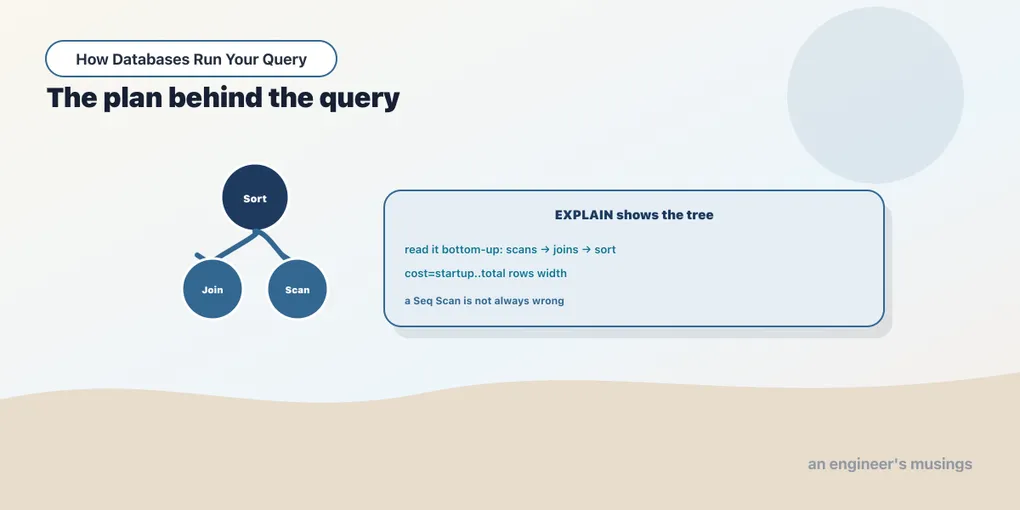
The first two series taught you to describe a result and let the database find it. This one is about the finding. When you hand Postgres a query, it doesn’t run your text; it compiles your text into a plan — a concrete sequence of physical operations — and runs that. Two queries that return the same rows can take a millisecond or a minute depending on the plan the database picked. Learning to read the plan is how you stop guessing about performance and start seeing it.
The tool is one keyword. Put EXPLAIN in front of any query and Postgres prints the plan it would run, without running it. That distinction matters: plain EXPLAIN costs nothing and touches no data. It shows you the strategy. The next chapter runs the query and measures reality; this one is about reading the strategy.
A plan is a tree
Start with the simplest useful shape, the per-genre summary from Series 1:
EXPLAIN SELECT genre, count(*), round(avg(price),2) FROM books GROUP BY genre; QUERY PLAN
---------------------------------------------------------------
HashAggregate (cost=16.50..16.59 rows=6 width=48)
Group Key: genre
-> Seq Scan on books (cost=0.00..12.00 rows=600 width=14)Two nodes, and the indentation is the whole grammar. A plan is a tree of operations, and each -> is a child feeding its parent. You read it bottom-up and inside-out: the deepest, most-indented node runs first, and its rows flow upward to the node above it.
Here the bottom node is a Seq Scan on books — a sequential scan, reading every row of the table in storage order. Those 600 rows flow up into the HashAggregate, which builds a hash table keyed by genre, accumulates the count and average per key, and emits one row per group. The reading order is the opposite of the printing order: the child at the bottom is where execution begins.
That inversion trips up everyone at first. The top line is the last thing that happens and the thing that produces your final rows. Everything below it is machinery feeding it.
The numbers on every node
Each node carries a parenthesized tag, and it is the same four numbers every time:
(cost=0.00..12.00 rows=600 width=14)costis two numbers, not one. The first is the startup cost: the estimated work before the node can emit its first row. The second is the total cost: the work to emit its last row. For a sequential scan startup is0.00, because it can return a row as soon as it reads one. For theHashAggregatestartup is16.50, nearly its total, because an aggregate has to consume all its input before it knows a single group’s count.rowsis how many rows the node expects to emit. The scan expects 600 (the whole table); the aggregate expects 6 (one per genre).widthis the estimated average row size in bytes.
The cost unit is arbitrary. It is not milliseconds and not any real-world quantity. By convention one unit is roughly the cost of reading one page sequentially from disk, and everything else is priced relative to that. What matters is not the absolute value but the comparison: the planner generates several candidate plans, prices each one, and keeps the cheapest. The cost is the currency it shops in. When you tune a query, you are trying to make the planner find a cheaper plan than the one it has.
Every number here is an estimate, computed from stored table statistics, before a single row is touched. Whether the estimates match reality is the subject of the next chapter, and the gap between them is where most performance bugs live.
The node types you will see constantly
The bookshop plans use a small vocabulary. Ask for a single row by primary key:
EXPLAIN SELECT * FROM orders WHERE order_id = 42; QUERY PLAN
---------------------------------------------------------------------------
Index Scan using orders_pkey on orders (cost=0.29..8.31 rows=1 width=21)
Index Cond: (order_id = 42)An Index Scan walks a B-tree index to jump straight to matching rows instead of reading the whole table. The Index Cond is the condition the index itself resolves. Total cost 8.31 against one row: cheap, and the subject of chapter 3.
Join two tables and a new node appears:
EXPLAIN SELECT b.title, a.name FROM books b JOIN authors a ON a.author_id = b.author_id; QUERY PLAN
-----------------------------------------------------------------------
Hash Join (cost=1.90..15.64 rows=600 width=23)
Hash Cond: (b.author_id = a.author_id)
-> Seq Scan on books b (cost=0.00..12.00 rows=600 width=18)
-> Hash (cost=1.40..1.40 rows=40 width=13)
-> Seq Scan on authors a (cost=0.00..1.40 rows=40 width=13)A Hash Join has two children. Read it bottom-up: the 40 authors are scanned and loaded into an in-memory Hash table keyed on author_id. Then the 600 books are scanned, and each book’s author_id is looked up in that hash to find its author. Building the hash from the smaller table and probing it with the larger is the classic strategy, and it has a whole chapter later in this series.
Sorting shows up as its own node:
EXPLAIN SELECT * FROM books ORDER BY price DESC; QUERY PLAN
---------------------------------------------------------------
Sort (cost=39.69..41.19 rows=600 width=40)
Sort Key: price DESC
-> Seq Scan on books (cost=0.00..12.00 rows=600 width=40)The Sort node’s startup cost (39.69) is almost its total, because a sort must see every input row before it can emit the first one in order. That startup-heavy signature is how a sort announces itself in the numbers.
Those five — Seq Scan, Index Scan, Hash Join, Sort, and an Aggregate node like HashAggregate — cover the large majority of everyday plans. Learn to spot them and most plans become readable.
When a full scan is the right answer
A sequential scan has a bad reputation it only half deserves. Reading every row is exactly correct when you want most of the rows. Count the whole orders table:
EXPLAIN SELECT count(*) FROM orders; QUERY PLAN
------------------------------------------------------------------
Aggregate (cost=1133.00..1133.01 rows=1 width=8)
-> Seq Scan on orders (cost=0.00..983.00 rows=60000 width=0)There is no index that helps here. To count every row you must visit every row, and reading them in storage order is the fastest way to do that. An index would be slower: it would bounce between the index and the table for all 60,000 rows, doing more work, not less.
The same holds for a filter that keeps a large fraction of the table:
EXPLAIN SELECT * FROM orders WHERE status = 'placed'; QUERY PLAN
-------------------------------------------------------------
Seq Scan on orders (cost=0.00..1133.00 rows=9940 width=21)
Filter: (status = 'placed'::text)About 9,940 of 60,000 orders are placed, roughly one in six. That is still too many for an index to pay off. The planner priced an index-based plan against this sequential scan and the scan won, so it chose the scan. A Filter line means “read the row, then test this condition and maybe discard it,” which is different from the Index Cond you saw earlier, where the index avoided reading non-matching rows at all.
The lesson worth carrying: a Seq Scan is not a symptom. On a small table, or a query that wants a big slice of a table, it is the planner making the right call. Panic is reserved for a Seq Scan on a large table where you expected only a handful of rows. Spotting that is what the rest of the series builds toward.
One portability note. Every database has an EXPLAIN, but the output is engine-specific. MySQL prints a table of rows rather than a tree (and EXPLAIN FORMAT=TREE gets you closer to this shape); SQLite’s EXPLAIN QUERY PLAN is terser still. The idea — the database compiling your query into a plan of physical operators — is universal. The exact words are Postgres’s.
Final thoughts
EXPLAIN prints the plan without running it: a tree of physical operators read from the bottom up, each tagged with cost=startup..total rows width. Costs are estimates in an arbitrary unit, used only to compare candidate plans and pick the cheapest. You now know the core node types and, just as important, that a sequential scan is often correct. What you have not seen yet is whether those estimates are any good. That is the difference between the plan the database thinks it will run and what actually happens when it does.
Comments