Estimates Versus Reality: EXPLAIN ANALYZE
EXPLAIN ANALYZE actually runs the query and prints what happened — real timings, real row counts next to the estimates, loop counts, and the buffer hits and reads that tell cache from disk. How to read the gap between guess and truth. Run against PostgreSQL 18.
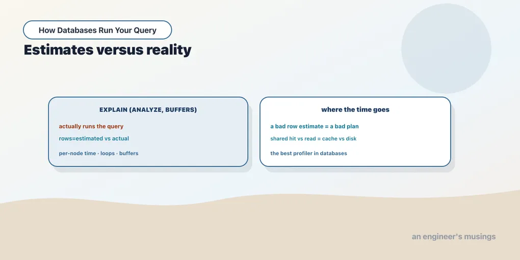
Plain EXPLAIN shows the plan the database intends to run, priced entirely from estimates. Estimates can be wrong, and a plan built on a wrong estimate is a slow plan. To see the truth you have to run the query and measure it. That is what EXPLAIN ANALYZE does: it executes the query and prints the plan annotated with what actually happened, next to what it predicted. Add BUFFERS and it also tells you how much of the work hit memory versus disk.
One caution before the first example: EXPLAIN ANALYZE runs your query for real. On a SELECT that is harmless. On an UPDATE or DELETE it will modify data, so wrap those in a transaction you can roll back. For the read-only bookshop queries here, we just run them.
Estimated next to actual
Take the sequential scan on order status from the last chapter and measure it:
EXPLAIN (ANALYZE, BUFFERS) SELECT status, count(*) FROM orders GROUP BY status; QUERY PLAN
-------------------------------------------------------------------------------------
HashAggregate (cost=1283.00..1283.05 rows=5 width=17)
(actual time=13.943..13.945 rows=5.00 loops=1)
Group Key: status
Batches: 1 Memory Usage: 32kB
Buffers: shared hit=383
-> Seq Scan on orders (cost=0.00..983.00 rows=60000 width=9)
(actual time=0.016..3.154 rows=60000.00 loops=1)
Buffers: shared hit=383
Planning Time: 0.387 ms
Execution Time: 14.073 msEvery node now carries a second parenthesis, the actual one, sitting right beside the estimate. Read them as a pair. The scan estimated rows=60000 and actually emitted rows=60000.00: a perfect match, because the whole table is 60,000 rows and Postgres knows it. The aggregate estimated 5 groups and got 5: there are five distinct statuses. When estimate and actual agree this closely, the planner was working from good information, and you can trust the plan it chose.
The actual time is two numbers with the same meaning as cost but in real milliseconds: time to the first row, then time to the last. The scan’s 0.016..3.154 says it produced its first row almost instantly and finished reading all 60,000 in about 3 ms. The aggregate’s 13.943..13.945 says it emitted nothing until 13.9 ms in, because it had to consume the entire scan before it knew any group’s count. At the very bottom, Execution Time is the real wall-clock total, and Planning Time is what the planner spent choosing the plan before execution even began.
One subtlety that saves confusion later: actual time is per-loop, and so is the actual row count. A node that runs many times reports its average time and rows, and you multiply by loops to get the true total. With loops=1 there is nothing to multiply, but that changes the moment a join is involved.
Loops, and multiplying them out
Join two tables on a small range of keys and the inner side runs repeatedly:
EXPLAIN (ANALYZE, BUFFERS)
SELECT o.order_id, c.name
FROM orders o JOIN customers c ON c.customer_id = o.customer_id
WHERE o.order_id BETWEEN 1 AND 20;
QUERY PLAN
---------------------------------------------------------------------------------------
Nested Loop (cost=0.57..147.33 rows=22 width=17)
(actual time=0.022..0.083 rows=20.00 loops=1)
Buffers: shared hit=63
-> Index Scan using orders_pkey on orders o (cost=0.29..8.73 rows=22 width=8)
(actual time=0.007..0.010 rows=20.00 loops=1)
Index Cond: ((order_id >= 1) AND (order_id <= 20))
Buffers: shared hit=3
-> Index Scan using customers_pkey on customers c (cost=0.28..6.30 rows=1 width=17)
(actual time=0.003..0.003 rows=1.00 loops=20)
Index Cond: (customer_id = o.customer_id)
Buffers: shared hit=60
Planning Time: 0.705 ms
Execution Time: 0.125 msA Nested Loop join takes each row from its first child and, for that row, runs its second child. The outer scan finds 20 orders. The inner scan on customers shows loops=20: it ran once per order, looking up that order’s customer by primary key. Its actual time=0.003 is the time for one lookup, not all twenty. Its rows=1.00 is one customer per loop. The real work of the inner side is 0.003 ms × 20 loops, and its buffer total confirms it: shared hit=60, which is roughly 3 buffers per lookup across 20 lookups. Forgetting the loops multiplier is the single most common misreading of an ANALYZE plan. A node that looks instant at 0.003 ms can dominate a query if it loops a hundred thousand times.
Buffers: cache versus disk
The BUFFERS option adds the line that turns a timing into an explanation. A buffer is one 8 KB page of a table or index. The line distinguishes two kinds:
shared hit— the page was already in Postgres’s cache (shared_buffers), served from RAM.shared read— the page was not cached and had to be fetched from the operating system, meaning disk or the OS page cache.
Every plan above showed shared hit only, because the bookshop is small and warm from earlier queries. To see a read, you need a cold cache. Immediately after restarting the server, the first scan of the largest table pays full price:
EXPLAIN (ANALYZE, BUFFERS) SELECT count(*) FROM order_items WHERE quantity >= 5; Aggregate (actual time=14.904..14.905 rows=1.00 loops=1)
Buffers: shared read=956
-> Seq Scan on order_items (actual time=14.901..14.901 rows=0.00 loops=1)
Filter: (quantity >= 5)
Rows Removed by Filter: 149942
Buffers: shared read=956
Execution Time: 15.089 msshared read=956: 956 pages fetched cold, and the whole thing took 15 ms. Run the identical query a second time and those pages are now cached:
   Buffers: shared hit=956
   ->  Seq Scan on order_items  (actual time=7.744..7.744 rows=0.00 loops=1)
 Execution Time: 7.796 ms
Same 956 pages, now every one a hit, and the time roughly halves. That difference — read on the first run, hit on the second — is the cache warming up. It is also why a query “feels slow the first time and fast after.” When you benchmark, run a query twice and compare the warm numbers, or you are measuring your disk, not your query. And notice Rows Removed by Filter: 149942: the scan read all 149,942 rows and threw every one away, because no order line has a quantity of 5. Work done to produce nothing is exactly the kind of thing an index exists to avoid.
When the estimate lies
So far estimate and actual have agreed. The interesting cases are when they don’t. Hide a column’s value from the planner behind a function:
EXPLAIN (ANALYZE, BUFFERS) SELECT * FROM customers WHERE upper(city) = 'LONDON'; Seq Scan on customers (cost=0.00..127.00 rows=25 width=52)
(actual time=0.091..1.979 rows=500.00 loops=1)
Filter: (upper(city) = 'LONDON'::text)
Rows Removed by Filter: 4500Estimated rows=25, actual rows=500.00: off by twentyfold. Postgres keeps statistics on the column city, and it knows London is a common value. But upper(city) is an expression it has no statistics for, so it falls back to a blind default guess of about 0.5% of the table (5000 × 0.005 = 25). Compare the plain-column version, where the stats apply:
EXPLAIN (ANALYZE) SELECT * FROM customers WHERE city = 'London'; Seq Scan on customers (cost=0.00..114.50 rows=500 width=52)
(actual time=0.012..0.502 rows=500.00 loops=1)
Filter: (city = 'London'::text)Estimated rows=500, actual 500: dead on. Same data, same 500 rows returned, but wrapping the column in upper() blinded the planner. Here the mistake is cheap, because both plans are a scan of a small table. On a larger query it is not cheap at all. A twentyfold underestimate is exactly how the planner talks itself into a nested loop that runs five hundred times instead of a hash join that runs once. A large gap between estimated and actual rows is the first thing to look for in a slow plan. It means the planner chose its strategy from bad information, and no strategy is reliable on bad information. Fixing the estimate — better statistics, or not hiding the column behind a function — often fixes the plan for free.
A note across engines: MySQL’s EXPLAIN ANALYZE (8.0.18 and later) prints a similar actual-versus-estimated tree, and SQLite has no direct equivalent. The Postgres habit of reading rows estimated against actual is the transferable skill; the exact syntax is not.
Final thoughts
EXPLAIN ANALYZE runs the query and annotates every node with actual time, rows, and loops, and BUFFERS splits the work into cached hit and cold read. Read actual against estimated on every node, remember that per-loop numbers multiply by loops, and treat a big estimate/actual gap as the prime suspect in a slow query. You have now seen the diagnosis. The rest of the series is treatment, and it starts with the single most effective one: the index that turns a full-table scan into a direct jump to the rows you asked for.
Comments