One Table, Many Pieces: Partitioning

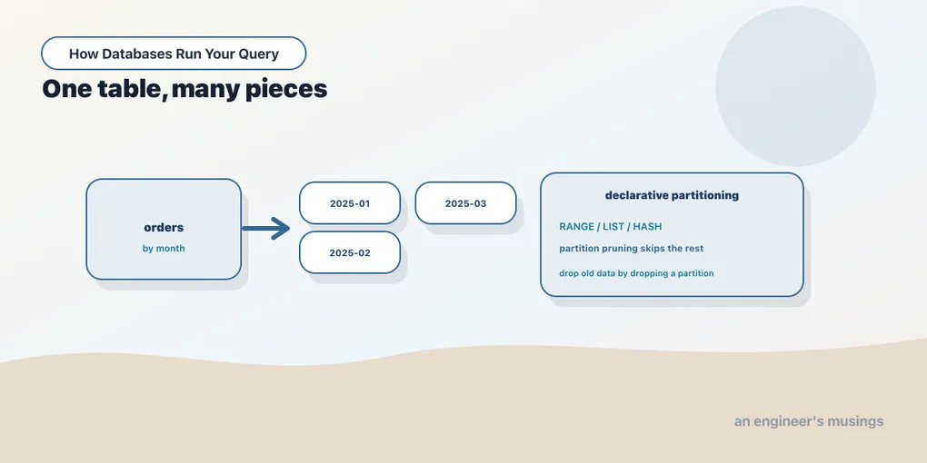
The last chapter fought bloat by cleaning one big table. This chapter takes a different tack: don’t keep one big table at all. Partitioning splits a logically single table into many physical pieces, each holding a slice of the rows, while queries and inserts still address it as one table. Done well, it buys three things. The database can skip whole slices that can’t contain your answer. It can delete a slice of old data in milliseconds. And each piece stays small enough that its indexes and vacuum stay cheap. The classic case is time-series data like our orders table, split by month.

Declaring a partitioned table

Postgres has had built-in declarative partitioning since version 10, and it’s the approach to use. You declare a parent table with a partitioning strategy and key, then attach child partitions that each own a range of that key. The parent holds no data itself; it’s a routing layer. I built a partitioned copy of orders in a scratch schema, keyed by order_date:

CREATE TABLE part.orders (
    order_id    int,
    customer_id int,
    order_date  date not null,
    status      text not null
) PARTITION BY RANGE (order_date);

That parent can’t store a single row yet, because no range is defined. Each partition claims a half-open interval, [from, to). Our data spans January 2023 through September 2025, so I created one partition per month, thirty-three of them. By hand each looks like this:

CREATE TABLE part.orders_2025_03
  PARTITION OF part.orders
  FOR VALUES FROM ('2025-03-01') TO ('2025-04-01');

The upper bound is exclusive, which is why adjacent months meet cleanly at the first of the month with no overlap and no gap. Creating thirty-three of these by hand is tedious, so in practice you generate them in a loop. A small DO block that walks a date forward a month at a time, issuing a dynamic CREATE TABLE ... PARTITION OF per iteration, is all it takes. That same loop, scheduled ahead, is how you provision next month’s partition before the data arrives. Then a single insert into the parent routes every row to the right child automatically:

INSERT INTO part.orders SELECT * FROM orders;   -- INSERT 0 60000

All 60,000 rows landed, each filed into its month’s partition by its order_date. You query part.orders exactly as you would any table; the partitioning is invisible to the SQL. What changes is what the planner does underneath.

Partition pruning: skipping the pieces

Here’s the payoff. When a query filters on the partition key, the planner can prove that most partitions can’t possibly match and refuse to even look at them. This is partition pruning. Ask for a single month, and after ANALYZE, the plan reads exactly one partition:

EXPLAIN (ANALYZE, COSTS OFF, TIMING OFF)
SELECT count(*) FROM part.orders
WHERE order_date >= '2025-03-01' AND order_date < '2025-04-01';

 Aggregate (actual rows=1.00 loops=1)
   ->  Seq Scan on orders_2025_03 orders (actual rows=1855.00 loops=1)
         Filter: ((order_date >= '2025-03-01') AND (order_date < '2025-04-01'))

One Seq Scan, on orders_2025_03 alone. The other thirty-two partitions weren’t scanned, weren’t opened, don’t appear in the plan. The planner did the interval arithmetic and pruned them before execution. A query spanning two months prunes to exactly two:

EXPLAIN (COSTS OFF)
SELECT count(*) FROM part.orders
WHERE order_date >= '2025-08-01' AND order_date < '2025-10-01';

 Aggregate
   ->  Append
         ->  Seq Scan on orders_2025_08 orders_1
         ->  Seq Scan on orders_2025_09 orders_2

The Append node stitches the surviving partitions together; here only August and September made the cut. Contrast that with a query that doesn’t filter on the key at all, such as one that filters only on status:

EXPLAIN (COSTS OFF) SELECT count(*) FROM part.orders WHERE status = 'shipped';

The plan is an Append over all thirty-three partitions, each with its own Seq Scan. With nothing to prune on, partitioning bought you nothing for this query, and arguably cost you a little overhead. That’s the central lesson: partitioning helps precisely when your queries filter on the partition key. Choose the key to match how you actually query, which for time-series data almost always means the date.

The other win: instant data lifecycle

Partitioning changes more than reads. Consider the common task of dropping old data, deleting every order before 2023. On a single table that’s a DELETE of thousands of rows, which writes just as many dead tuples for VACUUM to chase later, per the last chapter. On a partitioned table, the old month is its own table, so you drop the whole thing:

DROP TABLE part.orders_2023_01;   -- Time: 2.611 ms

Under three milliseconds, no dead tuples, no VACUUM aftermath. It’s a metadata operation, not a row-by-row delete. If you want to keep the data but remove it from the live set, perhaps to archive it, DETACH turns a partition back into a free-standing table:

ALTER TABLE part.orders DETACH PARTITION part.orders_2023_02;

After detaching February, the parent’s count dropped from 58,159 to 56,580. part.orders_2023_02 lived on as a standalone 1,579-row table you can archive or drop at leisure. This “roll off the oldest month, roll on a new one” rhythm is why partitioning and time-series data are such a natural fit. Rolling on is the mirror image: create next month’s partition ahead of time, and inserts start landing in it automatically.

Range isn’t the only strategy

RANGE is the workhorse, but two siblings round it out. PARTITION BY LIST assigns partitions by an explicit set of values, one partition per region or per status, say, rather than by an interval. PARTITION BY HASH spreads rows evenly across a fixed number of partitions by hashing the key. You reach for it when there’s no natural range or list but you still want to cap each partition’s size, say partitioning customers into eight buckets by customer_id. Range for time and ordered data, list for discrete categories, hash for even spread.

A few sharp edges worth knowing before you partition in anger. A UNIQUE constraint on a partitioned table must include the partition key, because Postgres enforces uniqueness per-partition, not globally. You can’t declare book_id alone unique across a table partitioned by date. Every partition inherits the parent’s indexes, but you create them on the parent and Postgres cascades them down. And partitioning adds planning overhead that grows with the partition count, so hundreds of partitions are fine and tens of thousands start to hurt. Keep the granularity sane: monthly or daily, not by the minute.

MySQL has its own PARTITION BY RANGE/LIST/HASH syntax baked into CREATE TABLE, similar in spirit though different in detail. SQLite has no native partitioning at all; the nearest idiom is separate tables glued together with a UNION ALL view, without the automatic routing or pruning.

Final thoughts

Partitioning turns one unwieldy table into many right-sized ones that still behave, to your SQL, as a single table. Two wins carry it. The planner prunes partitions a filter can’t match, so a one-month query scanned one partition out of thirty-three. And data lifecycle becomes a metadata operation, so dropping a month took under three milliseconds instead of a mass delete’s bloat. The catch is that pruning only fires when your queries filter on the partition key, so the key must match your access pattern. It’s the last of the structural tools in this series. Next we shift from restructuring data to reusing computed answers, and then to the query mistakes that quietly defeat everything you’ve learned.

Next: Cache the query, unlearn the traps — materialized views for expensive aggregates, and the anti-patterns that silently disable your indexes.