Understand the Cost of a Transformation
The report works on a small batch.
The report works on a small batch. To reason about a larger input, look at the state each operation must retain. The following experiment uses a separate generated JSON dataset and the recorded resource limits; it is not a benchmark of the XML report.
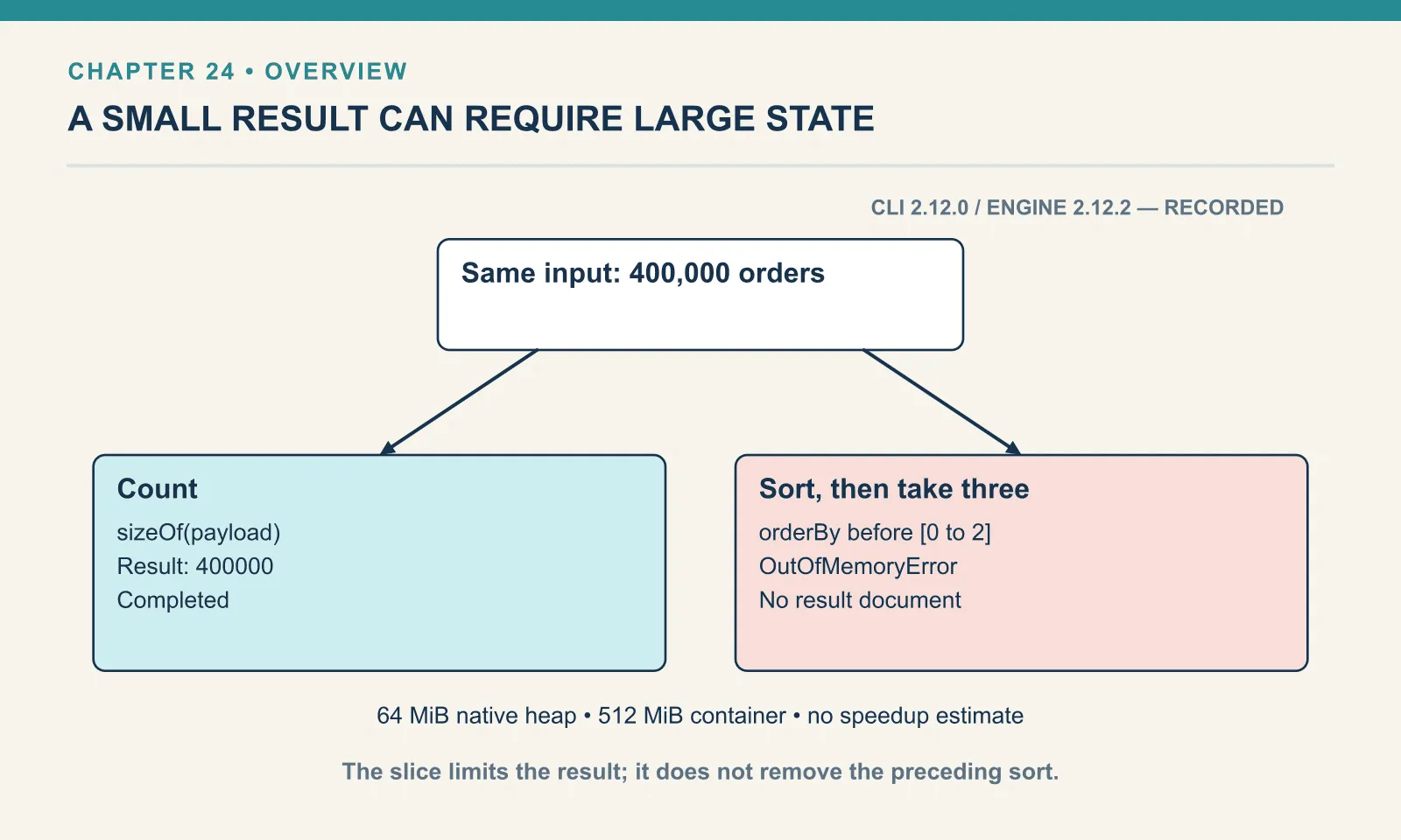
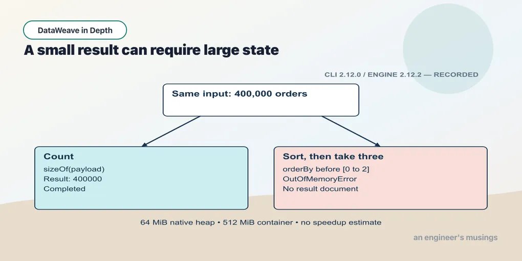
A count and a sort read the same file of 400,000 orders. The count returns 400000 under a 64 MiB heap limit. The sort fails with OutOfMemoryError under that same limit, even though its output asks for only three orders. Both scripts have streaming=true on their input. The setting is identical — what each expression needs to remember is not.
When a partner’s nightly export outgrows the sample file, the useful question is how much state must survive as the next order arrives. Counting can keep a number. Sorting must compare orders that may be anywhere in the input. Asking the writer for three results does not remove the work needed to discover which three come first.
The measurements in this chapter come from the book’s lab on DataWeave CLI 2.12.0, language runtime 2.12.2, using its Linux native executable in Docker. Each run saved its script, generated input, exit code and output. These are CLI measurements, not a Mule flow benchmark.
The numbered companion scripts use the five-order fixture for a quick functional check. The 400,000-order results and resource limits below are retained measurements from the original lab; running the small fixture does not reproduce those measurements.
Three places where memory can accumulate
An input file, an expression and a serialized result are different things. A reader turns bytes into values the expression can inspect. The expression computes new values. A writer encodes those values into bytes. Each stage can retain data, and each can postpone work until something asks for it.
For a line-by-line report, the expression might need only the current order. That does not establish how the input reached it or whether the output destination buffers the entire report. A connector can supply an already materialized value. A later operation can turn a manageable sequence into one enormous string. A consumer that wants the whole response before proceeding can erase the advantage of incremental production.
It is tempting to say that a reader without streaming always loads the entire document into heap. That is too strong. DataWeave also documents indexed readers for JSON, XML and CSV — an index and temporary disk storage allow access without retaining the whole document in memory, at the cost of disk activity and indexing work. Streaming reads move forward through the input’s records instead. These are distinct reader strategies, not interchangeable names for using less heap.
A modest heap graph does not reveal which reader strategy ran. The process might be streaming, using an index on disk, reading a small input, or evaluating only the part of the document a selector requested. Checking disk use and the actual result alongside memory helps distinguish those cases before attributing the behavior to one setting.
The directive uses equals signs
Here is the projection used in the small-input probe. It keeps three fields from each order:
Example 240 — Map a streamed five-order input.
Input payload — orders_five.json:
[
  {
    "orderId": "A-1001",
    "customer": "Dana",
    "items": [
      {
        "sku": "PEN-01",
        "price": 2.5,
        "qty": 1
      },
      {
        "sku": "PAD-22",
        "price": 6.0,
        "qty": 1
      }
    ],
    "total": 8.5
  },
  {
    "orderId": "A-1002",
    "customer": "Ravi",
    "items": [
      {
        "sku": "PAD-22",
        "price": 6.0,
        "qty": 2
      },
      {
        "sku": "CLP-08",
        "price": 1.0,
        "qty": 1
      }
    ],
    "total": 13.0
  },
  {
    "orderId": "A-1003",
    "customer": "Mei",
    "items": [
      {
        "sku": "CLP-08",
        "price": 1.0,
        "qty": 3
      },
      {
        "sku": "PEN-01",
        "price": 2.5,
        "qty": 1
      }
    ],
    "total": 5.5
  },
  {
    "orderId": "A-1004",
    "customer": "Tomas",
    "items": [
      {
        "sku": "PEN-01",
        "price": 2.5,
        "qty": 4
      },
      {
        "sku": "PAD-22",
        "price": 6.0,
        "qty": 1
      }
    ],
    "total": 16.0
  },
  {
    "orderId": "A-1005",
    "customer": "Dana",
    "items": [
      {
        "sku": "PAD-22",
        "price": 6.0,
        "qty": 5
      },
      {
        "sku": "CLP-08",
        "price": 1.0,
        "qty": 1
      }
    ],
    "total": 31.0
  }
]
%dw 2.0
input payload application/json streaming=true
output application/json
---
payload map (order) -> {
id: order.orderId,
buyer: order.customer,
total: order.total
}The five-order fixture holds the first five records the generator described below writes. Those orders reuse the book’s ID format, but their customers and totals are generated, so this A-1001 is not Dana’s three-line order totalling 32 from earlier chapters. The fixture produces:
[
  {
    "id": "A-1001",
    "buyer": "Dana",
    "total": 8.5
  },
  {
    "id": "A-1002",
    "buyer": "Ravi",
    "total": 13
  },
  {
    "id": "A-1003",
    "buyer": "Mei",
    "total": 5.5
  },
  {
    "id": "A-1004",
    "buyer": "Tomas",
    "total": 16
  },
  {
    "id": "A-1005",
    "buyer": "Dana",
    "total": 31
  }
]
streaming=true is a property on the input directive. Braces do not belong there, although the brace spelling looks natural to anyone who has passed options to read(). It fails to parse:
Example 241 — Reject object syntax in reader directives.
Use orders_five.json as payload, as above.
%dw 2.0
input payload application/json { streaming: true }
output application/json { deferred: true }
---
payload map (order) -> {
  id: order.orderId,
  buyer: order.customer,
  total: order.total
}
[ERROR] Error while executing the script:
[ERROR] Invalid input '{', expected options (line 2, column 32):
2| input payload application/json { streaming: true }
^
Location:
241-brace-syntax-fails (line: 2, column:32)The same mistake on an output directive fails too. The parser error is useful: it says the script never reached the stage at which it could choose a reader. Changing memory limits cannot repair a script that does not parse.
There is an object-shaped property syntax elsewhere, which helps explain the confusion. Chapter 18 passed reader options as the third argument to read. That argument is a DataWeave object:
Example 242 — Pass streaming options to read.
%dw 2.0
output application/json
var text = '[{"orderId":"A-1001","total":8.5},{"orderId":"A-1002","total":13}]'
---
read(text, "application/json", { streaming: true }) map $.orderId
[
"A-1001",
"A-1002"
]These forms occupy different grammatical positions. A directive takes options such as streaming=true; a function argument can be { streaming: true }. The second example also starts with an existing string. It demonstrates the option syntax, not a low-memory path from a multi-gigabyte source: the string has already been constructed before read receives it.
A reader’s streaming unit depends on the format. JSON commonly offers array elements; CSV offers records. XML needs a collection boundary, which the documented collectionPath property supplies. You have to place the reader configuration where bytes enter the flow. Putting it on one transform does not demonstrate that an earlier connector avoided buffering; the complete Mule path needs its own measurement. Streaming configuration
A writer that returns no bytes
The documented directive for deferred JSON output is:
Syntax fragment.
output application/json deferred=trueIn a Mule flow, the point is to let a later processor consume the output stream. It also changes where failures surface: work deferred until consumption can fail after control has left the Transform Message component. That matters when deciding which error handler can observe a conversion failure. A separate Mule 4.12.3 / Java 17 probe consumed deferred JSON through an HTTP Listener response on 13 September 2026. Two input orders produced the two expected projected objects, with HTTP 200 and chunked transfer encoding. This verifies consumption for that small flow; the late-error behavior remains documentation-based. Deferred output
The CLI result is more immediate. Adding deferred=true to the five-order projection produced empty stdout with exit code 0. Sending the result to a file also left a zero-byte file. The option parsed successfully, but no JSON document reached the destination. This is not an empty JSON array: [] is a document containing two bytes. It is no document at all.
So the measurements below use ordinary JSON output. A comparison can cover only the complete CLI paths that actually ran, and an empty file is no evidence that deferred writing is fast. The distinction is easy to lose when a benchmark records only elapsed time and whether the process exited successfully.
A reproducible check needs an expected result as well as an exit code. Compare a projection’s record count and selected values, or an aggregate’s value. With deferred output, also confirm that the consumer consumed the stream. These checks distinguish a completed report from a process that reported success without delivering one.
The large input and the limits
The generator creates a top-level array of 400,000 orders, totaling 54,920,574 bytes. Customer names cycle through Dana, Ravi, Mei and Tomas. Each order has two items and a numeric total; order IDs increase from A-1001, reusing the book’s ID format for generated orders rather than the running example’s. The inputs are deterministic, so a second run can compare the same records rather than a freshly randomized workload.
The constrained runs use a 512 MiB container limit and pass -Xmx64m to the native executable. Those limits describe different budgets. The native image heap is only part of the container’s memory. Native allocations, runtime bookkeeping and filesystem caching can contribute outside that heap.
The harness also saves cgroup memory.peak: peak container memory accounting, which can include page cache. It is not a precise measurement of the DataWeave heap or a process’s resident set alone. Treating it as either would make the table look more specific than the instrument permits.
Here are selected saved results from the constrained runs. Each row is from the second run except the three-reference row: that script ran only in the first, and a two-reference variant in the second run also exhausted the heap.
| Expression | Result with 64 MiB heap | Output |
|---|---|---|
payload[0].orderId | Completed | A-1001 |
sizeOf(payload) | Completed | 400000 |
Seeded reduce of order totals | Completed | 6333312 |
orderBy followed by selection of three results | Heap exhausted | No result document |
payload[-1].orderId | Heap exhausted | No result document |
groupBy $.customer, then a count per group | Heap exhausted | No result document |
Three separate references to payload | Heap exhausted | No result document |
The table describes these expressions on this executable and this fixture. It does not establish a general memory bound for every use of a selector, a fold or a reader. In particular, the fixture has small records. An incremental algorithm that retains one record can still struggle if one record contains an enormous string or a nested collection.
Counting consumes input without necessarily retaining it
The count script is deliberately small:
Example 243 — Count a streamed input.
Use orders_five.json as payload, as above.
%dw 2.0
input payload application/json streaming=true
output application/json
---
{ n: sizeOf(payload) }
Result on the five-order companion fixture:
{
  "n": 5
}
Its saved result was:
limit=512m xmx=64m exit=0
elapsed_s=12.9
peak_bytes=98582528
out_bytes=17
out_head={ "n": 400000}
A count has to reach the end of the input before it knows the final answer. That is a latency requirement, not proof that it must keep every preceding order. An implementation can advance a counter as it consumes records. The measurement does not expose DataWeave’s internal algorithm, but it does disprove the blanket claim that this expression necessarily holds the whole collection in heap.
The version without the streaming input directive also completed under the same heap limit. In the saved second run it took 40.7 seconds and reported 99,115,008 peak container bytes. The streaming version’s 12.9 seconds is one paired observation. In the first run the order was reversed: 5.9 seconds with the streaming directive and 5.6 without, at almost identical peaks of 93,765,632 and 93,675,520 bytes. Two paired runs that point in opposite directions are not a speedup estimate either way. Storage state, container startup, indexing and previous reads can affect the comparison. The important reproducible question here is whether both versions return the correct count within the specified budget.
The reversed timing order leaves no consistent multiplier to report. Estimating performance requires repeated runs, the same destination, a stated warm-up policy and enough samples to describe variation. The saved times remain useful observations, not a throughput guarantee, while the successful counts establish completion within the tested budget.
A fold is as small as its accumulator
The total uses the seeded fold from chapter 13:
Example 244 — Count with a streamed fold.
Use orders_five.json as payload, as above.
%dw 2.0
input payload application/json streaming=true
output application/json
---
{ revenue: payload reduce ((order, acc = 0) -> acc + order.total) }
Result on the five-order companion fixture:
{
  "revenue": 74
}
The constrained run returned:
limit=512m xmx=64m exit=0
elapsed_s=51.4
peak_bytes=94220288
out_bytes=24
out_head={ "revenue": 6333312}
The seed makes an empty input produce zero, and the accumulator retains a numeric total. The fold still visits every order. Its advantage is the state carried between visits, not skipping work.
A reduce that appends each order to an accumulating array has a different memory obligation. It retains an ever-growing result even though its traversal is forward-only. The function name does not decide whether the algorithm has bounded state. Inspect the accumulator and ask what it contains after the first record, after the thousandth, and after the last.
For grouped totals, the retained state depends on what each group holds. The table’s groupBy expression collects complete orders before counting them. Keeping one count per customer would retain less data, but that map would still grow with the number of distinct customers. With a unique customer ID on every order, it would grow with the input. Include distinct-key counts when estimating memory for a lookup.
Sorting before slicing still needs the sort
The report asks for the three largest orders:
Example 245 — Sort a streamed input.
Use orders_five.json as payload, as above.
%dw 2.0
input payload application/json streaming=true
output application/json
---
(payload orderBy -$.total)[0 to 2] map { id: $.orderId, total: $.total }
Result on the five-order companion fixture:
[
  {
    "id": "A-1005",
    "total": 31
  },
  {
    "id": "A-1004",
    "total": 16
  },
  {
    "id": "A-1002",
    "total": 13
  }
]
Under the constrained heap it failed before producing a result:
Exception in thread "main" java.lang.OutOfMemoryError: Garbage-collected heap size exceeded.
limit=512m xmx=64m exit=1
elapsed_s=2.0
out_bytes=0
The error line above is shortened; the full message goes on to suggest raising the maximum heap with -Xmx. orderBy must establish an order across the input before [0 to 2] can select the first three. The slice limits the output of sorting. It does not instruct orderBy to maintain only three candidates.
The failure shows that this expression exceeded this heap limit. It does not establish that every sorting implementation must keep all records in RAM: external sorting can use disk, and a dedicated top-k algorithm can retain a bounded candidate set. Neither alternative is what this script requested. If the upstream database can answer the ranking query, ask it to do so. If the transformation must own the ranking, choose and test an algorithm with the intended memory bound.
Grouping needs similar care. The table’s groupBy $.customer expression retains groups of orders and only then reduces each group to a count, and it exhausted the heap. Four customer names do not make those groups small: the arrays still contain 400,000 orders in total. A small final JSON object can hide a large intermediate value.
Access patterns matter more than their spelling
Selecting the first order completed under the small heap, returning A-1001. Selecting the last order exhausted it in the saved run. Both use an index selector, so if you treat all indexing as the same operation, you miss the useful difference.
The first element is available when the reader reaches it. The last cannot be identified until the reader knows where the sequence ends. That distinction explains why the expressions ask for different amounts of work; the measured memory outcome still belongs to this implementation. Do not infer from one failure that retaining the entire sequence is the only possible way to find its last element.
The multi-reference example requests the first ID, the total count, and a short projection from the same payload:
Example 246 — Read a streamed input more than once.
Use orders_five.json as payload, as above.
%dw 2.0
input payload application/json streaming=true
output application/json
---
{ first: payload[0].orderId, n: sizeOf(payload), ids: (payload map $.orderId)[0 to 2] }
Result on the five-order companion fixture:
{
  "first": "A-1001",
  "n": 5,
  "ids": [
    "A-1001",
    "A-1002",
    "A-1003"
  ]
}
It works on the small fixture but exhausts the constrained heap on the large one. The small run is useful for checking the output shape; it does not exercise the resource limit. References that look independent in the expression may require the runtime to retain or revisit data. Test the actual combination, not only each operation by itself.
When a report needs both detail rows and a total, decide where each result will be consumed. A single output object containing the entire detail array is a different delivery contract from a stream of rows followed by a separate summary. The consumer’s format can determine whether an otherwise incremental computation has to wait or buffer.
What the annotation establishes
One more probe runs a function whose parameter carries @StreamCapable:
Example 247 — Declare a stream-capable parameter.
Use orders_five.json as payload, as above.
%dw 2.0
input payload application/json streaming=true
output application/json
fun summarise(@StreamCapable orders) =
  orders map (o) -> { id: o.orderId, total: o.total }
---
summarise(payload)
Result on the five-order companion fixture:
[
  {
    "id": "A-1001",
    "total": 8.5
  },
  {
    "id": "A-1002",
    "total": 13
  },
  {
    "id": "A-1003",
    "total": 5.5
  },
  {
    "id": "A-1004",
    "total": 16
  },
  {
    "id": "A-1005",
    "total": 31
  }
]
Both the bare annotation and the @StreamCapable() spelling parsed in the saved probes. In the saved second run against the 400,000-order file, the bare-annotation version completed under the 64 MiB heap and wrote 18,939,623 bytes. That demonstrates accepted syntax and the result of this particular function. It does not demonstrate that annotating any function will catch every hidden allocation or transform it into a streaming implementation.
MuleSoft documents a separate experimental validation pattern using @StreamCapable() on an input directive. It checks access restrictions, including repeated references and negative indexing. Those validation checks are not a profiler. A result can satisfy an access rule and still be expensive because of the size of a record or the state retained by a later operation. Conversely, a validator may reject a pattern whose particular fixture happens to work. The input-directive validation behavior was not exercised by the parameter-annotation probes in this chapter. Stream validation
Use the annotation for the contract the tooling actually checks, and a large, representative input to establish resource behavior. Neither substitutes for the other.
What was not run
The separate Mule HTTP probe verified a small deferred response, not performance or bounded memory. XML collection streaming at scale, repeatable-stream strategies, disk-spill limits and deferred-writer error handling remain unrun. The CLI measurements and the Mule response test answer different questions.
The saved measurements cover one generated dataset and a specific native executable. They do not establish production concurrency, network throughput, backpressure through a flow, worst-case record sizes or disk usage. The cgroup measurement does not isolate heap occupancy. The CLI’s acceptance of streaming=true also does not prove which internal strategy every operation ultimately used.
These limits identify the next experiment: a Mule test that reads the fixture through the intended connector, consumes the output through the intended destination, asserts the result, and records both heap and temporary disk behavior. Repeat the run with a late invalid record and a slow consumer. A pipeline that is fast until an error occurs has not yet demonstrated the failure behavior an operator needs.
Exercises
1. A successful empty file. The deferred transform exits successfully, but its output file is empty. Has the performance test passed?
Show answer
No. Exit code zero is insufficient evidence. The fixture should produce five projected orders, and a zero-byte file contains no JSON document. Verify a consumer actually consumed the result and compare the output before timing it. For this pinned CLI, use ordinary output for a working projection and keep the small Mule consumption test separate from unmeasured performance and error behavior.
2. Three results, whole sort. Why does selecting three entries after orderBy still fail with a small heap?
Show answer
The slice applies to the sorted result. The script first asks orderBy to establish the ordering across all orders. Limiting the number of emitted records does not bound that intermediate operation. An upstream ranking query or a separately implemented and verified top-k algorithm changes the computation; moving a slice after the existing sort does not.
3. One fold is not every fold. A count succeeds under the small heap. Can you now promise that every reduce is safe on a large file?
Show answer
No. Inspect the accumulator. A numeric count retains a number; an array accumulator that appends every input retains the collection. A map of customer counts grows with the number of distinct customers. The useful bound is the retained state, including any unusually large record, rather than the name of the higher-order function.
Final thoughts
The count, fold and sort all read the same orders. Their resource requirements differ because their intermediate results differ. A memory investigation becomes productive when you identify what must survive the next record and then measure the path from source bytes to a consumed, checked result. A property accepted by the parser is the start of that work. The output and the failure case tell you whether it succeeded.
A checked result, the actual input and the complete consumption path belong in a performance experiment. Keep those alongside the measurement so that a successful process with no delivered document cannot be mistaken for a faster transformation.
Comments