A Document in a Column: JSON and JSONB
Storing and querying semi-structured data inside a relational database — why jsonb beats json, the access operators, shredding a document into rows and building rows back into a document, containment and path queries, and where a GIN index fits. Run against PostgreSQL 18.
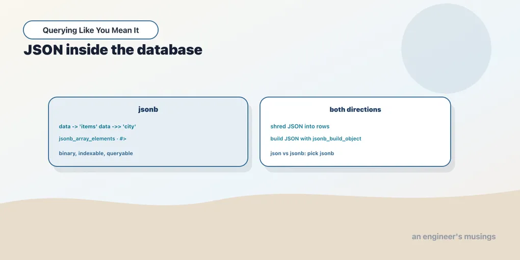
The relational model wants every value to be scalar: one typed thing per cell, no lists, no nested structure. That rigidity is the source of most of SQL’s power. But real data doesn’t always arrive that way. An API returns a nested object, a webhook payload has optional fields that differ row to row, an event log carries a bag of attributes you can’t enumerate in advance. Postgres answers this with a JSON column type, so you can keep a whole document in one cell and still query into it with SQL. This chapter is about doing that well, which starts with picking the right type.
json vs jsonb: always jsonb
Postgres has two JSON types, and the choice is nearly always the same. json stores the exact text you gave it, whitespace and all. jsonb parses the document once, on the way in, and stores a binary representation. That parse has three visible consequences: keys get deduplicated (last value wins), key order is not preserved, and insignificant whitespace disappears. Watch the same literal become two different things:
SELECT '{"b":1, "a":2, "a":3}'::json  AS as_json,
       '{"b":1, "a":2, "a":3}'::jsonb AS as_jsonb;
as_json | as_jsonb
-----------------------+------------------
{"b":1, "a":2, "a":3} | {"a": 3, "b": 1}
(1 row)json kept the text verbatim, duplicate a and all. jsonb dropped the duplicate ("a": 3 won), reordered the keys, and normalized the spacing. The binary form costs a little more to write but far less to read, because querying it doesn’t re-parse text every time. And only jsonb can be indexed for containment and existence. Use jsonb unless you have a specific reason to preserve the original bytes exactly, which is rare. Everything below uses jsonb.
Reaching in: the access operators
There are four operators for pulling values out, and the split that trips people up is object-versus-text. -> returns a jsonb value; ->> returns text. The path forms #> and #>> do the same, but take an array path so they can dig several levels deep in one step.
SELECT j ->  'title'              AS arrow,
       j ->> 'title'              AS arrow_text,
       j #>  '{author,country}'   AS path,
       j #>> '{author,country}'   AS path_text
FROM (SELECT '{"title":"Dune","author":{"name":"Herbert","country":"USA"}}'::jsonb AS j) t;
arrow | arrow_text | path | path_text
--------+------------+-------+-----------
"Dune" | Dune | "USA" | USA
(1 row)Notice arrow came back as "Dune" with quotes (it’s still jsonb, a JSON string) while arrow_text is bare Dune (plain text). That distinction matters the moment you compare or cast: to test country = 'USA' you want ->>, the text form. To keep drilling deeper, you want ->, so the result is still jsonb you can subscript again. The path operators save you from chaining: j #>> '{author,country}' is j -> 'author' ->> 'country' written flat.
Shredding a document into rows
A document with an array inside it is the classic mismatch: one row holds many things. To bring those things back into the relational world you shred the array into rows with jsonb_array_elements (or _text for text output). Here’s a small scratch table of book documents, each with a tags array:
CREATE SCHEMA scratch;
CREATE TABLE scratch.docs (id int, doc jsonb);
INSERT INTO scratch.docs VALUES
 (1, '{"title":"Dune","genre":"Sci-Fi","price":42,"tags":["epic","desert","spice"]}'),
 (2, '{"title":"Emma","genre":"Fiction","price":19,"tags":["classic","romance"]}'),
 (3, '{"title":"Sapiens","genre":"Nonfiction","price":28,"tags":["history","epic"]}');

SELECT d.id, tag
FROM scratch.docs d,
     jsonb_array_elements_text(d.doc -> 'tags') AS tag
ORDER BY d.id, tag;
id | tag
----+---------
1 | desert
1 | epic
1 | spice
2 | classic
2 | romance
3 | epic
3 | history
(7 rows)Three documents became seven rows, one per tag, each still carrying its document’s id. That comma-join to a set-returning function is an implicit LATERAL join — the next chapter covers it in full. For now, read it as “for each row, expand its array into rows.” Once shredded, the data is ordinary rows, so ordinary aggregation applies. Tag frequency across the corpus:
SELECT tag, count(*) AS docs
FROM scratch.docs, jsonb_array_elements_text(doc -> 'tags') AS tag
GROUP BY tag
ORDER BY docs DESC, tag;
tag | docs
---------+------
epic | 2
classic | 1
desert | 1
history | 1
romance | 1
spice | 1
(6 rows)To walk an object’s keys instead of an array’s elements, jsonb_each yields one (key, value) row per top-level field:
SELECT key, value FROM scratch.docs, jsonb_each(doc) WHERE id = 2 ORDER BY key; key | value
-------+------------------------
genre | "Fiction"
price | 19
tags | ["classic", "romance"]
title | "Emma"
(4 rows)Querying without shredding: containment and paths
Sometimes you don’t need to expand the array, you just need to ask whether it contains something. The containment operator @> tests whether the left document contains the right one, arrays included. Documents tagged epic:
SELECT id, doc ->> 'title' AS title
FROM scratch.docs
WHERE doc -> 'tags' @> '["epic"]'
ORDER BY id;
id | title
----+---------
1 | Dune
3 | Sapiens
(2 rows)No jsonb_array_elements, no join, just “does this array contain epic.” For richer queries there’s the SQL/JSON path language via jsonb_path_query. In it, $ is the document root, .key navigates, and ? (@ > 25) filters:
SELECT id, jsonb_path_query(doc, '$.price ? (@ > 25)') AS price
FROM scratch.docs
ORDER BY id;
id | price
----+-------
1 | 42
3 | 28
(2 rows)Only the two documents whose price cleared 25 produced a row. Path queries get expressive quickly (wildcards, array slices, arithmetic), and they read cleanly for the deep, conditional lookups that would otherwise be a stack of ->.
Building rows back into JSON
The reverse direction is just as useful: take relational rows and assemble a JSON document, usually to hand to an API. jsonb_build_object(k, v, ...) makes one object, and jsonb_agg folds many objects into an array, honoring ORDER BY inside the aggregate.
SELECT jsonb_agg(
         jsonb_build_object('title', doc ->> 'title',
                            'price', (doc ->> 'price')::int)
         ORDER BY (doc ->> 'price')::int
       ) AS catalog
FROM scratch.docs;
catalog
-----------------------------------------------------------------------------------------------------
[{"price": 19, "title": "Emma"}, {"price": 28, "title": "Sapiens"}, {"price": 42, "title": "Dune"}]
(1 row)Three rows collapsed into one JSON array, price-ascending. This works over the real tables too. jsonb_object_agg(key, value) builds a single object from a two-column result, which turns a grouped summary into an API-ready payload in one shot:
SELECT jsonb_object_agg(genre, n) AS by_genre
FROM (SELECT genre, count(*) AS n FROM books GROUP BY genre) g;
by_genre
----------------------------------------------------------------------------------------------------
{"Poetry": 100, "Sci-Fi": 100, "Fiction": 100, "History": 100, "Children": 100, "Nonfiction": 100}
(1 row)The whole genre breakdown, one object. Between jsonb_agg, jsonb_build_object, and jsonb_object_agg, you can shape query output into whatever document a caller expects, without leaving SQL.
Indexing, and a note on portability
On performance: a WHERE doc @> '...' filter over a large table can use a GIN index on the jsonb column (CREATE INDEX ON t USING gin (doc)). That turns containment and key-existence lookups into fast index probes instead of a scan over every document. That indexability is the strongest practical reason to prefer jsonb over json.
On portability, JSON support is the most dialect-specific corner of SQL. The binary jsonb type, the @> containment operator, GIN indexing, and jsonb_path_query are Postgres. MySQL has a single JSON type (already binary, no separate jsonb) and uses ->/->> plus functions like JSON_EXTRACT and JSON_CONTAINS; SQLite has json1 functions such as json_extract. The concepts carry over, but assume every function name and operator here needs translating when you leave Postgres.
Final thoughts
JSON in the database is the pressure valve for data that won’t sit still in columns. The discipline is to use it deliberately, not as a dumping ground. Choose jsonb for the binary storage and the index. Then learn the two directions. Shred documents into rows with jsonb_array_elements and jsonb_each when you want to filter, join, and aggregate. Build documents from rows with jsonb_build_object and jsonb_agg when you need to hand structure back out. And when you only need to test membership, @> and the path language answer without expanding anything. The relational model and the document model aren’t enemies here; jsonb is the seam where they meet. Next we take the array type seriously in its own right, and meet the join that lets a subquery see the row it’s attached to.
Comments